Visualising Entropy
Our quest to find the tile index of D-Sat 1 continues. I have described before, what I mean with “tile index” and I have also given a clue that I found something in the first part of the big blob of data dsatnord.mp which I named un1.dat.
In this post we will
- extract the byte offsets of the tiles from
dsatnord.mp, - search for those byte offsets in the unknown parts of
dsatnord.mp, and - analyse the found data.
This post is based on a Jupyter Notebook which contains the code to repeat the analysis.
Apart from a much better understanding of how tiles are stored and accessed in D-Sat 1, our visually most appealing outcome is this picture:
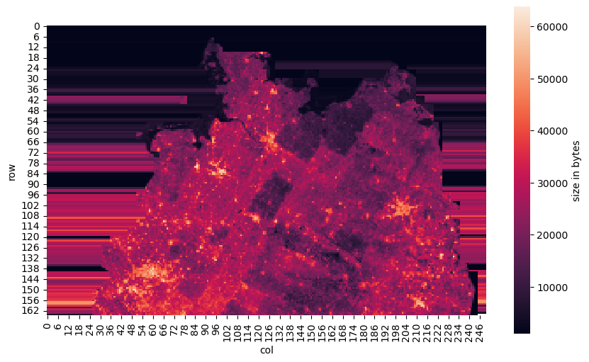
You might recognise some known shape but wonder what the colours indicate. We will come to that but for now let’s just say that the image is proof of the (at least partial) solution to the quest of finding the tile index.
This post describes the journey towards getting (and understanding) that image in very much detail. Thus, it is rather long and probably contains too much information for some – and still, there are bits and pieces missing. For example, many of the visualisations shown here were only produced after looking at the data in other formats (hex values, integer values, etc.)
Extracting the byte offsets of the tiles
As described before,
we are looking for information about the tiles that contain the
satellite images. Since the tiles are stored sequentially in
dsatnord.mp, the most simple way to identify them is their byte
offset
within that file. If an index describing the tiles exists, that index
likely contains the offsets of the tiles as pointers (integer
numbers). Thus, we first extract those offsets from dsatnord.mp
using the gen_offsets function in
mp.py.
Searching for the byte offsets
Now we can search within dsatnord.mp for individual offsets to find candidate parts for the index. We can restrict our search to the three parts whose function we do not know, yet, and we start with the first part un1.dat, ranging from byte 0 to byte 316020 in dsatnord.mp.
How can we search for the offsets? One approach is to start with a handful of (randomly chosen) offsets.
random_offsets = tiles.sample(5).offset.to_list()
random_offsets
[30243192, 616207380, 203431531, 496386351, 376324742]
Then there are two options to search for them: either we transform the
offsets into byte values or we transform the bytes of the target file
into integers. I chose the second approach. In both cases we need to
decide how to represent an integer, which basically requires us to
settle the parameters of
int.from_bytes:
number of bytes, byte order, and whether the value has a sign or
not. Given the size of dsatnord.mp (644833911 bytes), two bytes (16
bit) are clearly not sufficient, so the next typical choice is 4 bytes
(32 bit). To represent (absolute) offsets we do not need a sign and
little endianness is the typical byte order of the
hardware D-Sat was
running on.
So we want to check all successive four bytes in the first part of dsatnord.mp, but we can not be sure that the index starts at byte 0. The simplest thing to do then is to just take every byte position and check the integer formed by the successive four bytes:
with open("../dsatnord.mp", "rb") as f:
    for pos in range(316020):
        f.seek(pos)
        lint = int.from_bytes(f.read(4), byteorder='little', signed=False)
        if lint in random_offsets:
            print("found offset", lint, "at byte position", pos)
found offset 30243192 at byte position 7756
found offset 203431531 at byte position 90504
found offset 376324742 at byte position 130820
found offset 496386351 at byte position 155140
found offset 616207380 at byte position 176132
That looks good! Some more analysis revealed that actually all tile offsets are contained in the first part un1.dat. Furthermore, there are (almost) no gaps between offsets, that is, (almost) each successive 4 byte integer represents an offset of a tile. This also means that this index does not contain any coordinates! This was quite unexpected and the reason why I continued searching for the index, although I already knew that un1.dat contains the offsets.
Last but not least, the first offset starts at byte 16, so I assume the first 16 bytes of dsatnord.mp constitute the file header, which looks as follows:
50 31 32 00 44 53 41 54 98 34 01 00 f2 2d 0f 00 |P12.DSAT.4...-..|
Analysing the data
Now we want to understand how the index is structured. Therefore, we first read the offsets into a dataframe:
| un1off | offset | |
|---|---|---|
| 0 | 16 | 316020 |
| 1 | 20 | 328719 |
| 2 | 24 | 351371 |
| 3 | 28 | 384572 |
| 4 | 32 | 405841 |
| ... | ... | ... |
| 78996 | 316000 | 644833911 |
| 78997 | 316004 | 644833911 |
| 78998 | 316008 | 644833911 |
| 78999 | 316012 | 644833911 |
| 79000 | 316016 | 3650133385 |
79001 rows × 2 columns
Does this make sense? Let us again have a look at the number and sizes of tiles we have found:
| start offset | end offset | tile size | number of tiles |
|---|---|---|---|
| 316020 | 1070097 | 250x250 | 20 |
| 1070097 | 10127037 | 500x500 | 169 |
| 16194771 | 86822577 | 500x500 | 2240 |
| 86822577 | 644833451 | 1000x1000 | 24701 |
| sum: 27130 |
The 79001 numbers are way more than the 27130 tiles we have found. To better understand what is going on, let us plot the data:
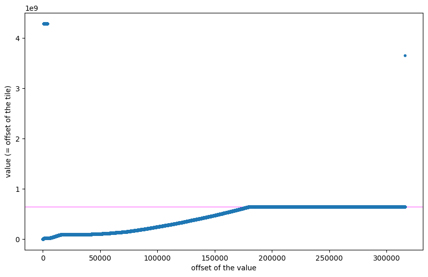
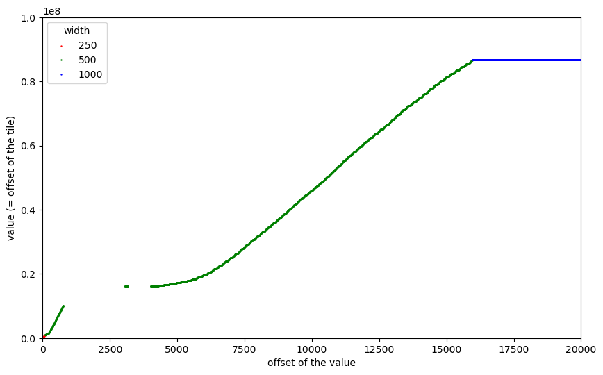
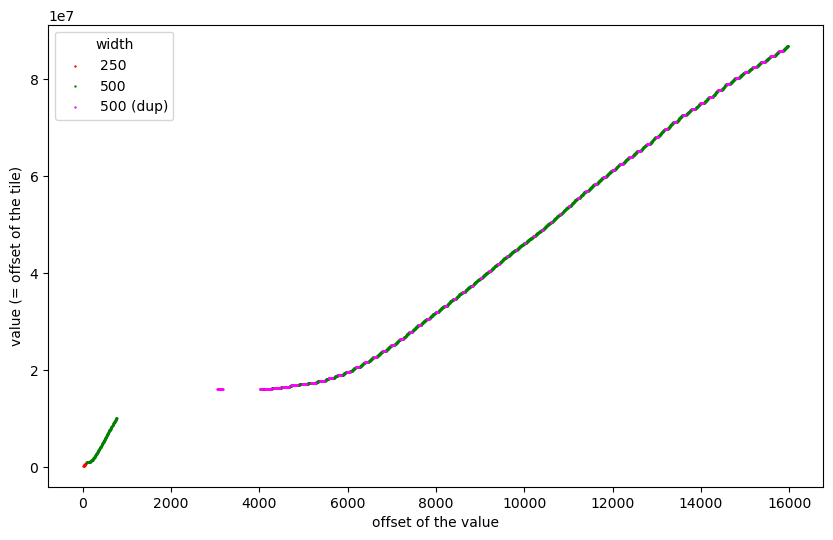
The horizontal axis shows the actual offset of each value at the beginning of dsatnord.mp (i.e., the part I call un1.dat). The vertical axis shows each value found at that offset and we interpret these values as offsets (pointers) into dsatnord.mp, that is, the offsets of the tiles.
The magenta line depicts the actual size of dsatnord.mp, so at the beginning and at the end there are clearly some values that can not be offsets into dsatnord.mp. The (roughly) first half contains increasing values and the second half (almost?) constant values. We cannot see from this plot which values are actually offsets of the tiles, but we can join the data with the actual offsets of the tiles and visualise that:
| un1off | offset | size | width | height | |
|---|---|---|---|---|---|
| 0 | 16 | 316020 | 12699.0 | 250.0 | 250.0 |
| 1 | 20 | 328719 | 22652.0 | 250.0 | 250.0 |
| 2 | 24 | 351371 | 33201.0 | 250.0 | 250.0 |
| 3 | 28 | 384572 | 21269.0 | 250.0 | 250.0 |
| 4 | 32 | 405841 | 40818.0 | 250.0 | 250.0 |
| ... | ... | ... | ... | ... | ... |
| 78996 | 316000 | 644833911 | NaN | NaN | NaN |
| 78997 | 316004 | 644833911 | NaN | NaN | NaN |
| 78998 | 316008 | 644833911 | NaN | NaN | NaN |
| 78999 | 316012 | 644833911 | NaN | NaN | NaN |
| 79000 | 316016 | 3650133385 | NaN | NaN | NaN |
79001 rows × 5 columns
The undefined (NaN) values for size, width, and height at the end show that these are not offsets of tiles. We can now colour the points in the plot according to tiles of which size they represent:
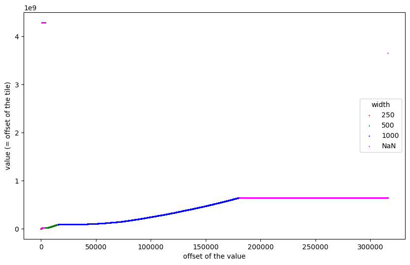
Hardly visible are the 20 tiles of size 250x250 at the beginning, which are followed by 169 tiles of size 500x500 which are also hardly visible. Then follow some outliers, 2240 tiles of size 500x500, and 24701 tiles of size 1000x1000. The second half of the file does not contain offsets of tiles.
Clearly, it is interesting to understand the purpose of the values I have called “outliers” but for now let us skip them:
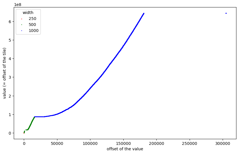
That is the plot I started pondering about a lot. It turned out that at this scale it is difficult (if not impossible) to get an understanding of what we see (and why). So I started to zoom into some regions (actually, using interactive plots enabled by %matplotlib notebook):
We can now see the 250x250 tiles at the very beginning, the first 169 tiles of size 500x500, the gaps caused by outliers, and then a “staircase”-like distribution of the remaining 2240 tiles of size 500x500. Let us further zoom into the first part before the gaps:
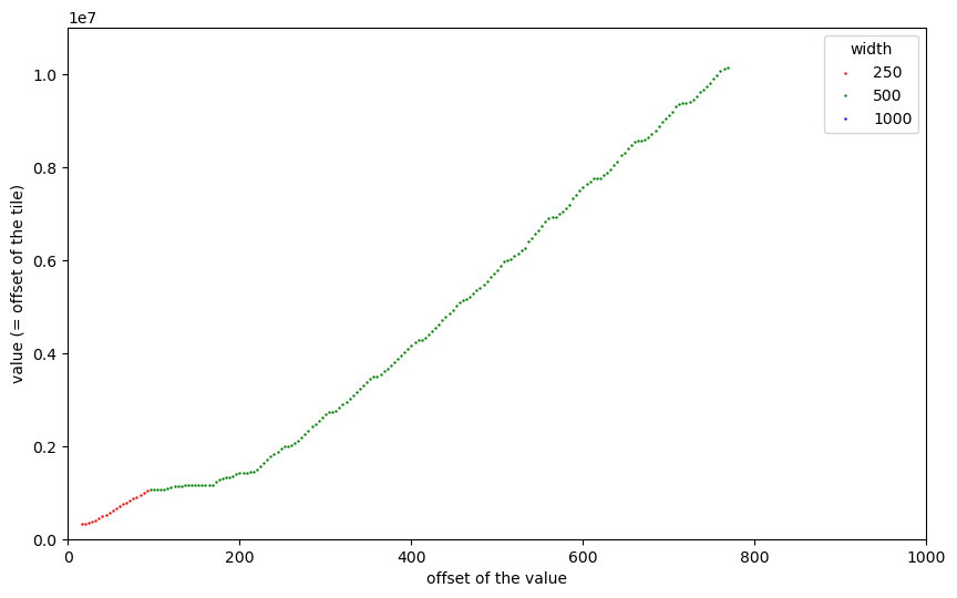
Now we can see a “staircase” pattern also for the first 169 tiles of size 500x500. Remember, that the tiles in dsatnord.mp are (almost all) stored adjacently without any gaps and that the vertical axis shows their byte offsets. So the flat parts of the curve are caused by tiles that occupy not much memory. That was one very important observation towards understanding how the tiles are ordered.
But why should the tiles have vastly different memory sizes? After all, they represent squares with the same side length. The reason must be the compression ratio: some tiles could be better compressed. And the reason for that must be that the image they show must have a lower entropy, that is, could be easier compressed. In our case of satellite images the reason could be that the landscape they show is rather “dull”, for example, a body of water.
In the meantime, I had also extracted and converted the 20 tiles of size 250x250 and checked how they were arranged: basically in a grid of 5 rows and 4 columns, stored in row-major order starting from the top left corner.
Combining this information together with the thoughts about the memory sizes of tiles, I decided to plot their byte size in a heatmap with the tiles arranged in a 5 by 4 grid:
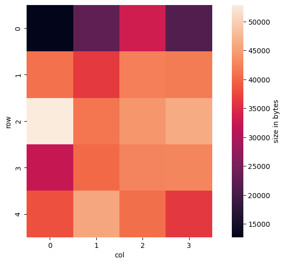
We can see that the upper left tile does not occupy much memory. That is because it shows almost only the North Sea (which I confirmed by looking at the actual image) which is almost completely blue without any structure and thus can be compressed very well. Actually, most of the tiles in row 0 cover sea and thus could be compressed very well.
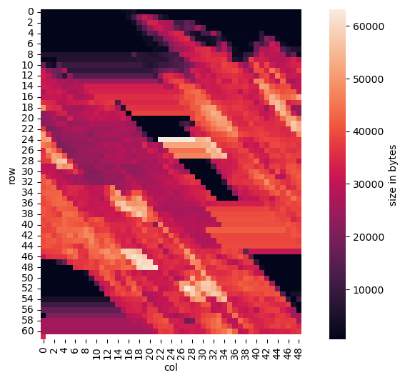
So let us have a look at the next zoom level. We need to figure out how the 169 tiles of size 500x500 could be arranged. Since 169 = 13 * 13, we try 13 rows and 13 columns:
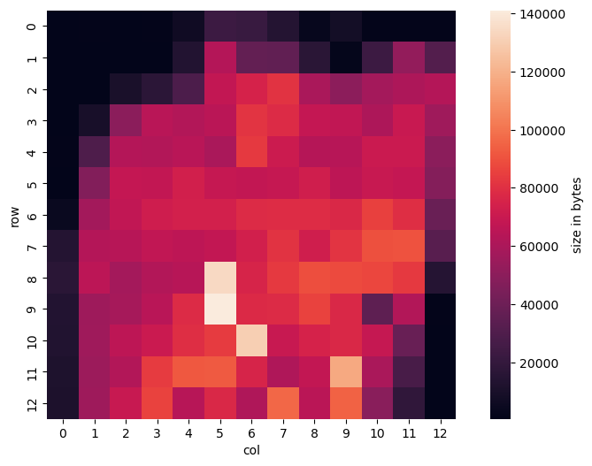
Columns 0 and 12 look as if something has been cut off but the north could resemble the coastline of Germany.
Now we could just continue zooming in using the remaining tiles, but before I did that, I made another observation: the frequency distribution of tile offsets clearly showed that several offsets were repeated. So let us plot the offsets of the 250x250 and 500x500 tiles only and highlight duplicate values in magenta:
We can see quite some duplicates and, apparently, they are the reason for the staircase effect in the 2240 tiles of size 500x500.
When zooming in, we can observe a similar effect for the 1000x1000 tiles:
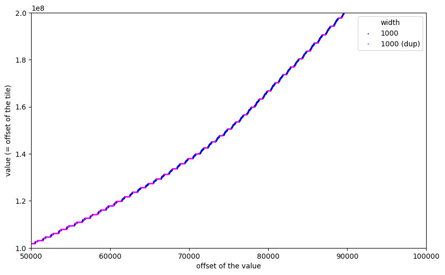
And these were the plots which kept me awake. I thought: if this is really the tile index, why are some tiles repeated? And why is there this regular but changing pattern of repetitions and non-repetitions?
In such situations it helps to have someone else have a look and brainstorm what this could be. And as with the magic number for the tiles, my colleague Jan helped a lot to form the following hypothesis: The repeated tiles fill the area outside Germany to form a rectangle.
This would mean that I could just continue plotting the tiles in a rectangular grid without any need to know the shape of Germany. That came somewhat as a surprise and showed some simplicity that I did not expect.
So the next zoom level would be the remaining 2240 tiles of size 500x500. However, my first tries did not work and I got a garbled image. Having a look at one of our initial plots, we can see that at offset 3052 the offset 16194771 for the first 500x500 tile is repeated 30 times and then there is a gap (from bytes 3172 to 4012) filled with the “outlier” value 4278772525. So let us skip this first (repeated) tile and use only the tiles from byte 4016 to byte 15972. This makes 2989 = (15972 − 4016) / 4 (repeated) tiles which can be factored into 7 * 7 * 61. So one guess could be to use a grid of 7 * 7 = 49 columns and 61 rows:
We can clearly see some shearing distortion, which means we did not choose the right number of columns. So the best guess is to try adjacent values and having started with 49, 50 is one next best choice:
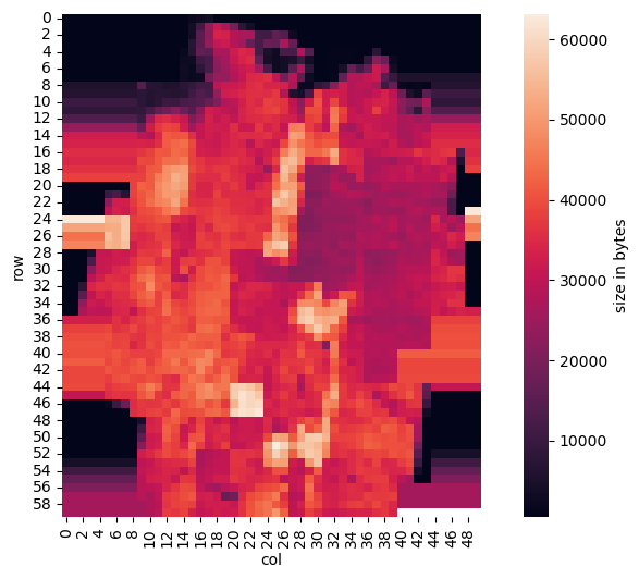
That looks familiar, doesn’t it? The coast line of Germany is clearly visible. The vertical stripes outside of Germany are caused by the repetition of the “border” tiles, that is, the last tiles east and west that cover Germany. By not storing tiles that do not cover Germany, precious space could be saved on the CD-ROM. And by just repeating the border tiles, programming was simplified, since the shape of Germany was not required to load tiles – they tiles are just arranged in a rectangular grid.
What we can also see is that so far all tiles cover the whole of Germany although we are analysing tiles from the first CD-ROM covering only the north of Germany. This will be different for the tiles of size 1000x1000 with the highest resolution (I spare you a detour and directly show you the correct result with 250 columns which I found as second guess after 200 columns):
I hope you are as astonished as I was when I first saw that image. This definitely shows the north of Germany – the coastline and even the inland shape is clearly identifiable. Beyond this, there are more things to observe and explain:
- The horizontal bars east and west outside Germany are (again) caused by the repetition of the border tiles.
- We only see the northern half, since the southern half is stored on
the second CD-ROM in the file
dsatsued.mp. Although we have not analysed that file so far, it is almost certain that it is structurally the same asdsatnord.mp. - Although the colour of each pixel just indicates the byte size of the 1000x1000 pixel tile at that location, we can clearly see some structure. In particular, we can identify the Ruhr area in the west and several large cities, for example, Hamburg, Bremen, Hannover, Berlin, and Dresden. The reason for that is that the plot basically visualises entropy: images of the complex structure of streets and houses in cities have a higher entropy and thus can not be compressed as well as low-entropy images of fields, meadows, and woods. How well data can be compressed is related to its entropy.
- Particularly in the middle of the image we can see “traces” of larger patches going from the bottom to the top in an angle of roughly 60° (measured from the bottom). My hypothesis is that these are caused by the orbit of the satellite who took the images. Depending on the weather (and other) conditions over a region during flyover, the quality of the images might be different, causing different entropy.
So we now know how the tiles are arranged and that there is basically a(nother) “pixel coordinate system”. What is missing is information on how to translate between those and well-known coordinate systems and projections. From a pessimistic point of view this means we are not much farther with our knowledge than from the first post. However, today I would like to take the optimistic point of view and state that we have already reverse-engineered a very big part of the file format of D-Sat 1.