Finding something unexpected
After having visualised the “uncharted” parts of
dsatnord.mp our quest to
find the index for the tiles continues.
Before we start, let me briefly explain what I mean with “index for the tiles” and what I expect to find: the satellite images of Germany consist of individual tiles that the viewer shows when zooming into a specific region. To find the correct tile for a geographic area, there must be an index that provides some coordinates for each tile. My assumption is, that for each (quadratic) tile the index contains a coordinate for a fixed position of the tile, for instance, for the lower left corner. Visualising those coordinates for all tiles would yield a lattice pattern with the shape of Germany – something like this but much denser:
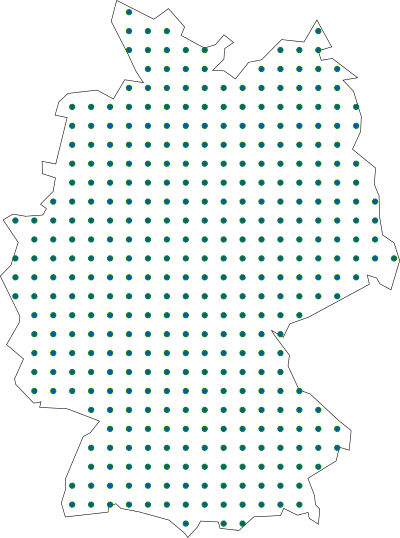
Of course, other technical solutions would be thinkable. Specifically, there is no need to use the lower left corner or a fixed position at all for that matter. However, we need some hypothesis to start with and that is mine.
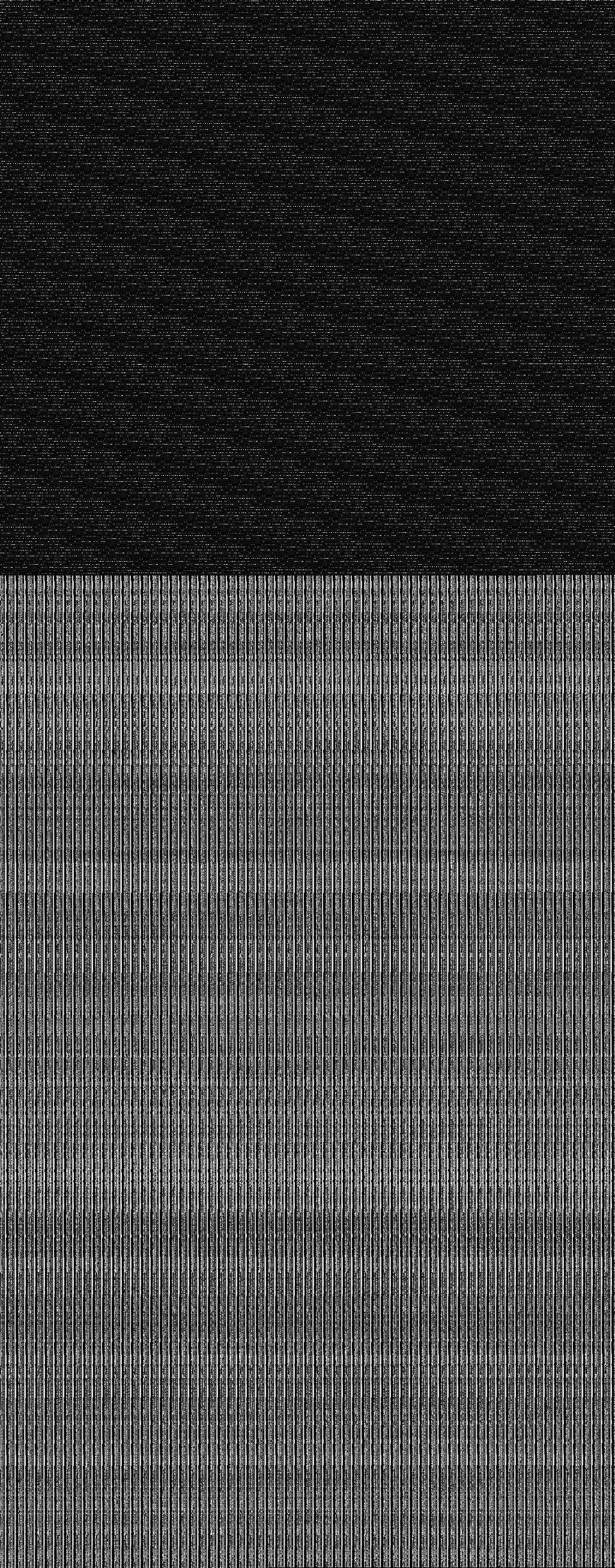
So let us have a look at the unknown parts of dsatnord.mp to search
for the tile index. Most promising looks the third part (un3.dat),
since it clearly consists of two parts, each revealing a periodic
pattern:
(Spoiler alert: before I analysed that part I actually had a closer
look at the first part un1.dat and found data that is related to the
tiles but I will report that later, since I consider the find
described here more remarkable.)
My first goal was to find the byte offset in un3.dat where the first
part ends and the second begins. Using Gimp, I found that the second
part begins roughly in row 957 (of 2610) and column 890 (of 1024).
Since each pixel represents one byte, that translates into the byte
offset 1024 * 957 + 890 = 980858. Since un3.dat has 2672062 bytes
overall, this is roughly at 37%, which fits with the image. To get
multiples of 16, I shortened the second part by 4 bytes, that is, from
offset 980858 to offset 980862 (we will later see why that makes
sense):
dd if=un3.dat of=un3_1.dat bs=4M count=980862 iflag=count_bytes
dd if=un3.dat of=un3_2.dat bs=4M skip=980862 iflag=skip_bytes
Again, we can visualise the results to check whether we split the file correctly:
./src/mp.py -c vis_bytes -o un3_1.png un3_1.dat
./src/mp.py -c vis_bytes -o un3_2.png un3_2.dat
The results (not shown here) look good.
Now my assumption was that the index contains a record (with the
coordinates and possibly other information) of fixed length for each
tile. I started with the second part (un3_2.dat) since it showed
quite some regularity and performed different analyses to test that
hypothesis. Among those were:
- Creating successive n-byte ints/floats and visualising their
correlation using
seaborn.pairplot. (This could have led me to the result but it did not work with the whole part such that I used just the first 10kB of the data which was not enough to recognise a pattern.) - Measuring distances between successive n-byte ints/floats and visualising their distribution using histograms (not really helpful) and scatterplots. (The motivation behind that analysis was that tiles of equal size should have approximately equally spaced coordinates, resulting in approximately the same distances between coordinates. The results were some weird patterns which indicated that there must be something regular.)
- Visualising the distribution of the byte values. (I saw some spikes but could draw no real conclusion.)
I did some more analyses along those lines but have not documented them well, so this post focuses on the successful path, something which I had in mind the whole time: computing the autocorrelation between byte values, to find the size of each record. My assumption was that the index consists of records for the tiles and each record has a fixed structure which results in the repeating pattern we saw initially. Autocorrelation can help us to find the frequency of the pattern and thus the record length. Here’s what I did:
reading the bytes into a dataframe
from struct import unpack
import pandas as pd

with open("../un3_2.dat", "rb") as f:
    vals = []
    while ((data := f.read(1))):
        vals.append(int.from_bytes(data, byteorder="little", signed=False))

df = pd.DataFrame(vals, columns=["ints"])
computing and plotting the autocorrelation
import statsmodels.tsa.stattools as smtsa
import numpy as np

acf = smtsa.acf(df.ints, nlags=100, adjusted=False, fft=False)

lags = np.arange(len(acf))
plt.rcParams['figure.figsize'] = (10, 5)

plt.vlines([6, 10, 16], -0.2, 0.8, color="lightgrey")
plt.plot(lags[1:], acf[1:])
plt.xlabel("bytes")
plt.xlim(xmin=0)
plt.ylabel("correlation")
plt.show()
The result looks as follows:
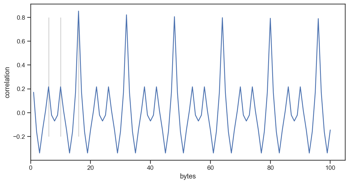
We can see a high correlation at 16, meaning there is a repeating pattern every 16 bytes. So that is likely our record size.
Now I built a dataframe with 16 columns: each containing one record per row such that each byte is represented as an integer value in each column.
from struct import unpack
import pandas as pd

bytelen = 16

with open("../un3_2.dat", "rb") as f:
    vals = []
    while ((data := f.read(bytelen))):
        vals.append([int.from_bytes(data[i:i+1]) for i in range(bytelen)])

df = pd.DataFrame(vals, columns=["i" + str(i) for i in range(bytelen)])
Next, I was analysing the different columns, for example, checking
their
value_counts. I
saw that some columns (that is, byte positions) contain only very few
(e.g., 1, 2, or 3) different values and others contained all possible
256 byte values. I skip some details here but the next plot (plus the
raw numbers) gave me a clue how to proceed:
fig, ax = plt.subplots(4)
for i in range(4):
    df["i" + str(i)].hist(bins=256, ax=ax[i])
    ax[i].set_xlim(0, 256)
plt.show()
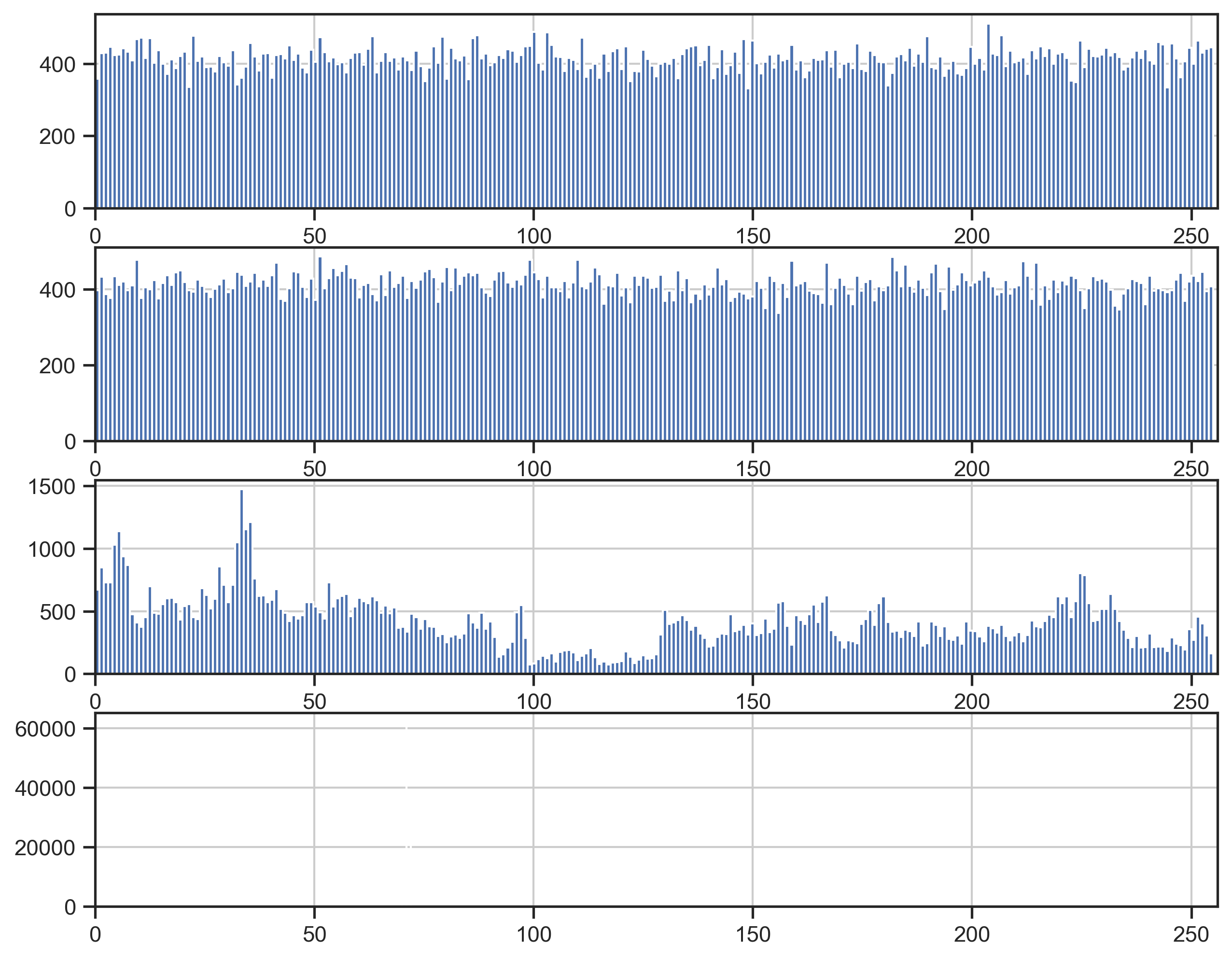
Byte 0 looks random, byte 1 looks random, byte 2 looks much less random and byte 3 contains only three different values (71, 72, 70 with frequencies 62076, 39222, 4402, respectively – unfortunately not visible in the plot). My guess was that these are the four bytes of a number in little endian order, because the least significant bits (i.e., the first two bytes) would show high variation but the most significant bits should be more limited, as the coordinates are restricted to Germany.
I saw a similar pattern with bytes 4 to 7, so I read the first 8 bytes into two 32 bit integers (little endian, unsigned) and visualised them in a scatter plot:
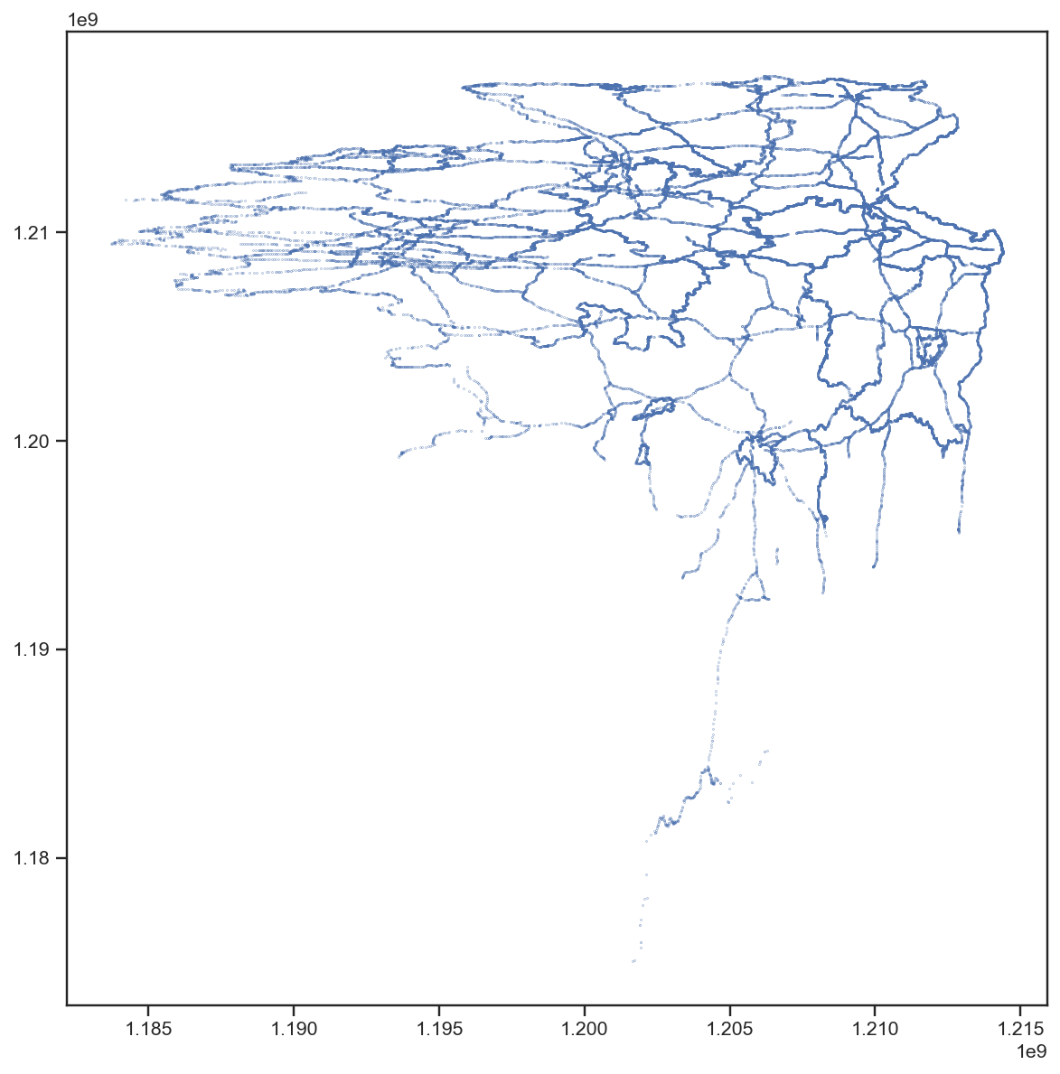
Surprised? Any idea, what this could be?
Well, that’s definitely not the tile index, I thought. But it’s also definitely not random. It looks like lines … polygons … maybe … wait a second. Let’s turn this by 180° (and use floats instead of ints, although that came one step later):
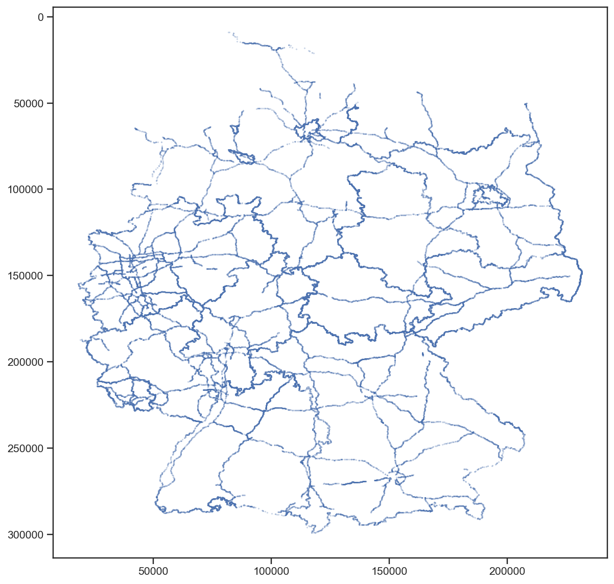
The borders of the states of Germany and the main highways!
Since we have just decoded the first 8 bytes of the 16 byte record, the remaining bytes certainly encode more information. For example, byte 13 has just three distinct values with the following frequencies:
| value | frequency |
|---|---|
| 1 | 43150 |
| 0 | 38260 |
| 2 | 24290 |
So it is safe to assume that it encodes three different things. Assigning the colours red, green, and blue to 0, 1, and 2, respectively, we get the following map:
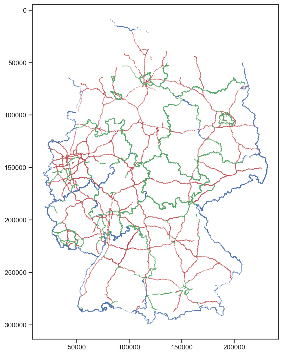
(I fixed the distortion with plt.gca().set_aspect('equal').)
So 0 seems to encode highways, 1 state borders, and 3 the border of Germany (with some exceptions mainly in the west).
Although for the part un3_2 we analysed here there are still 7 bytes
left to decode for each record, overall, this is a big step forward to
fully understand the structure of dsatnord.mp. So even though I have
(again) not found the tile index (yet), I am very happy about this
finding. It was also kind of unexpected, since the D-Sat 1 CD-ROM
contains a file dsat.vec which contains strings like “A100” and
“A10/E30” which are clearly names for highways. Thus I assumed that
this vector data is (only) contained in that file but that is
apparently not the case.
Most of my analyses are contained in this Jupyter Notebook.