Fragmenting the tile data
When looking at the data segment of CIS/COD
images (i.e., the
tiles) the byte sequence 0x63 0x6f 0x64 (ASCII: cod) appears
several times and thus is conspicuous. According to a wiki page
describing a derived video
codec
it marks the end of a “plane”, a basic building block of
wavelet-compressed images. In this post we explore the size
distribution of these blocks.
Let us start by analysing how many such parts we find in images for the different tile types:
20 colour tiles of size 250x250
| number of parts | frequency |
|---|---|
| 39 | 17 |
| 42 | 2 |
| 48 | 1 |
169 colour tiles of size 500x500
| number of parts | frequency |
|---|---|
| 36 | 162 |
| 39 | 7 |
2240 colour tiles of size 500x500
| number of parts | frequency |
|---|---|
| 36 | 2238 |
| 37 | 1 |
| 39 | 1 |
24700 greyscale tiles of size 1000x1000
| number of parts | frequency |
|---|---|
| 13 | 24667 |
| 14 | 33 |
We can clearly see that tiles from the same type have mostly the same number of parts: typically 36 for colour tiles and 13 for greyscale tiles (with the exception of the 250x250 overview tiles which have mainly 39 parts).
Without going into further detail (yet) I can state that each part likely represents a “sub-band” of the wavelet decomposition which has a certain depth for each component (e.g., colour). The most simplest case are the greyscale tiles where we have 13 parts which would fit nicely to the following sub-band structure of depth 4:
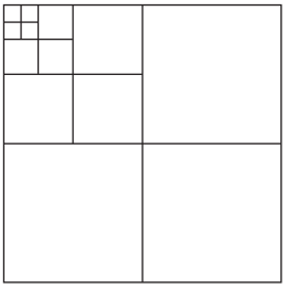
(Given the depth d, the number of sub-bands can be computed as 3d + 1.)
The following plot shows the size distribution of the components over all greyscale 1000x1000 tiles for each sub-band:
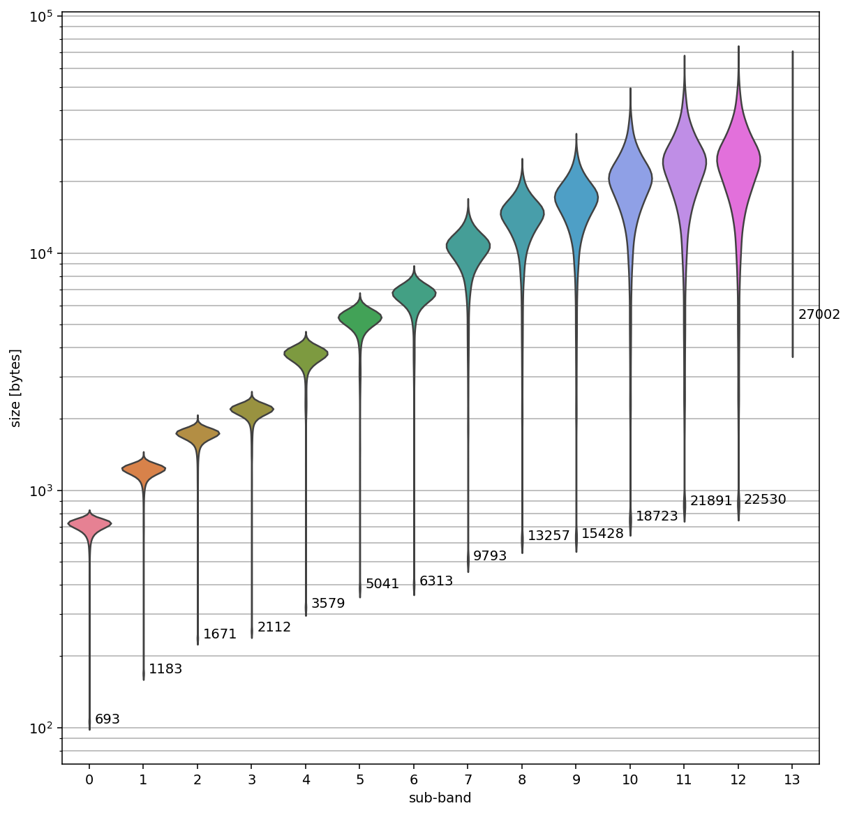
The vertical axis is scaled logarithmically and the numbers at each lower end of the violin plot indicate the mean for each sub-band.
We can see that the size required for each sub-band increases from (on average) 693 bytes for sub-band 0 to (on average) 22530 bytes for sub-band 12 (excluding sub-band 13 which only 33 images have). This nicely fits the typical order in which sub-bands in wavelet compressed images are stored: The first sub-band provides a very much scaled-down version of the original image. Successively adding information from the following sub-bands improves the image quality step-by-step by adding more details which supports progressing loading and display of images.
For comparison, here’s the plot for the 2240 colour tiles of size 500x500:
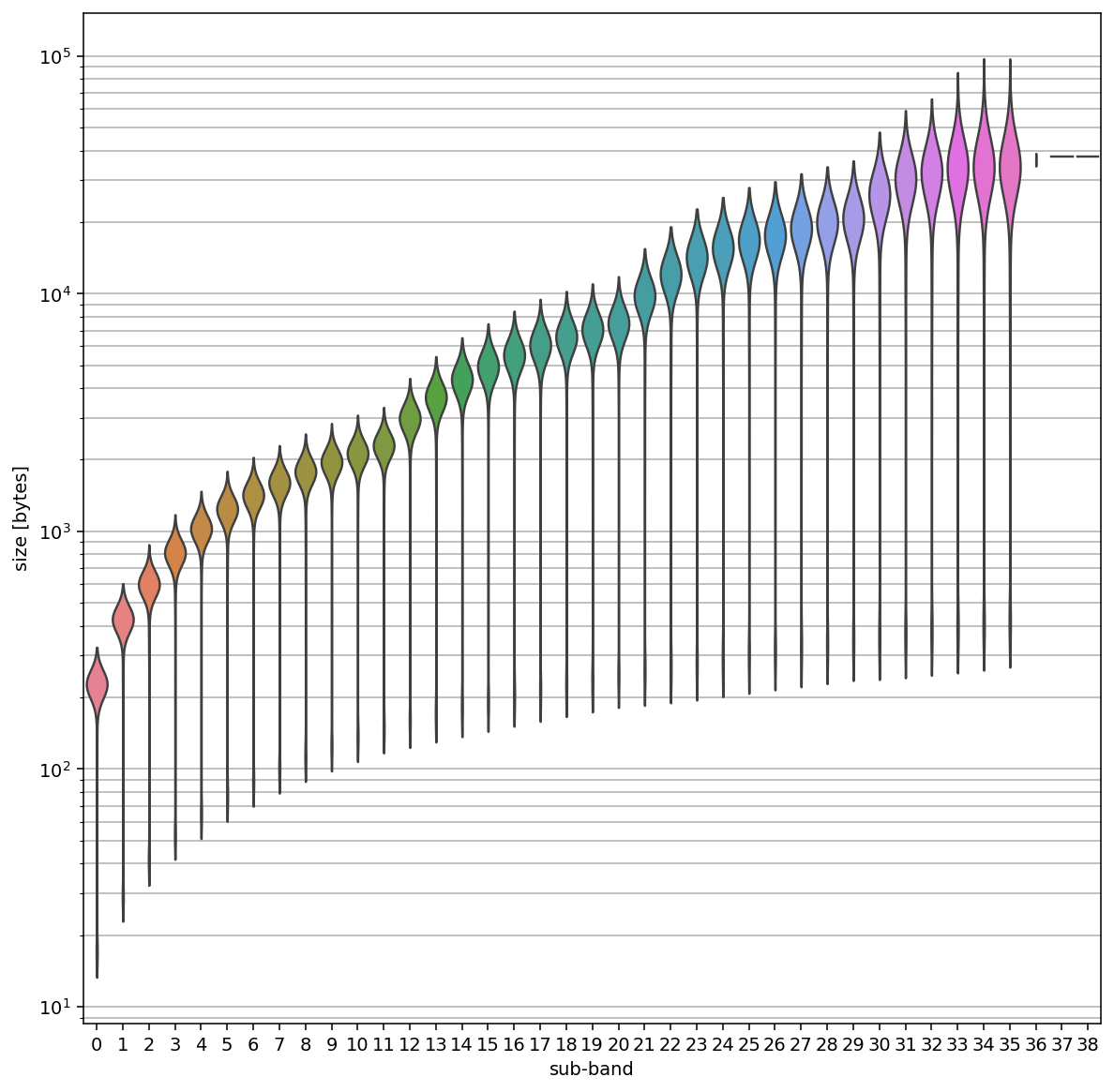
Most of these tiles have 36 parts that represent encoded sub-bands – which does not fit to the abovementioned formula. However, we also have colour images, thus three components (probably YCbCr). I suppose that the Y component (luma) is encoded in more detail (= higher depth) than the colour components. For example, instead of having the same depth of 4 for all three components, a depth of 5 for luma and a depth of 3 for Cb and Cr each would result in the observed 36 sub-bands (3 * 5 + 1 + (2 * (3 * 3 + 1)).
This Jupyter Notebook contains the code to create the plots from this post. A good starting point for further reading is Chapter 16 “Wavelet-Based Image Compression” of the book Introduction to Data Compression by Khalid Sayood.